59. Net extCable feature

The identification tag for this tutorial is PDS-ACJ. Pregenerated input files for this tutorial are found in the folder named PDS-ACJ in the provided tutorial input files.

59.1. Tutorial overview

This tutorial covers:

Net arrays
Net integrated rib lines

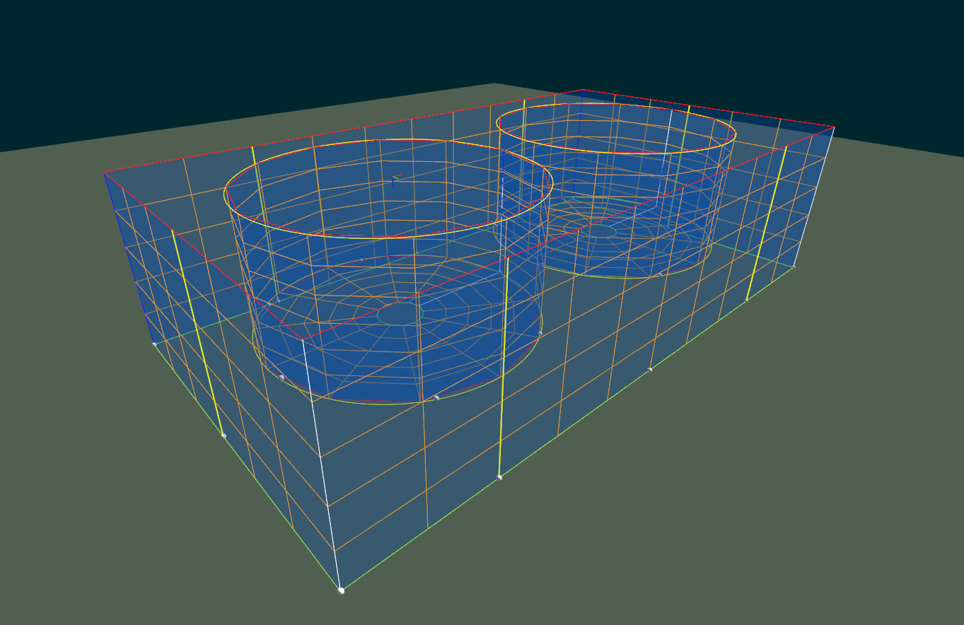
Fig. 59.1 Net integrated rib lines

59.2. Create a predator net panel

Note

Integrated rib lines in nets significantly reduce the number of DObjects and connections required, as cable DObjects are not required to be created for netting rib lines.
Integrated rib lines will be added to a basic predator net, which will be added to the Cylindrical net cage array tutorial.

Create a copy of the input folder for the Cylindrical net cage array tutorial.

Note

If the Cylindrical net cage array tutorial has not been completed, the required input files can be downloaded here .

Create a new net DObject called PredatorNet_1.
Set node (0,0)’s position to (-20,20,0) m.
Set node (0,N)’s position to (55,20,0) m.
Set node (M,0)’s position to (-20,20,20) m.
Set node (M,N)’s position to (55,20,20) m.
Define the number of elements between node (0,0) and node (0,N) to be 10.
Define the number of elements between node (0,0) and node (M,0) to be 5.
Set edge 0 to be static with $Edge0Static 1 in the PredatorNet_1 input file.

Note

Once the net is created the rib lines can be added as an extra cable feature.

Add 4 longitudinal rib lines by adding the following lines into the net input file: $ExtCableLongitudinal segment0 0, $ExtCableLongitudinal segment0 15, $ExtCableLongitudinal segment0 60, and $ExtCableLongitudinal segment0 75.

Note

The ExtCables on the edges are not shown in the visualizer in order to preserve the edge color definitions.
To model the lateral rib lines, the $ExtCableTransverse can be used in a similar fashion.
Rib lines are commonly used to support clump weights placed at the bottom of the net.

Add a 0.5 m diameter and 2400 kg/m³ density spherical extmass named clump to the bottom of each ribline.

Note

The PredatorNet_1 input file should look like the following:

// Boundary constraints
$Node00Static 0
$NodeM0Static 0
$Node0NStatic 0
$NodeMNStatic 0
$Edge0Static 1
$Edge1Static 0
$Edge2Static 0
$Edge3Static 0
$Edge2Ring 0
$Edge0Ring 0

// Hydrodynamic
$FluidCoefficientReData reynoldsDependentNetDragData

// Mechanical
$NetPanelProperties dNetPanel

$ExtMass clump 0 20
$ExtMass clump 15 20
$ExtMass clump 37.5 20
$ExtMass clump 60 20
$ExtMass clump 75 20



$ExtCableLongitudinal segment0 0
$ExtCableLongitudinal segment0 15
$ExtCableLongitudinal segment0 60
$ExtCableLongitudinal segment0 75

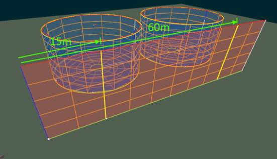
Fig. 59.2 Longitudinal ExtCable example

59.3. Add the rest of the predator cage

Duplicate PredatorNet_1 with a -40 m offset in the Y direction.
Rename the duplicate net as PredatorNet_2.
Create a new net DObject called PredatorNet_3.
Set node (0,0)’s position to (-20,-20,0) m.
Set node (0,N)’s position to (-20,20,0) m.
Set node (M,0)’s position to (-20,-20,20) m.
Set node (M,N)’s position to (-20,20,20) m.
Define the number of elements between node (0,0) and node (0,N) to be 6.
Define the number of elements between node (0,0) and node (M,0) to be 5.
Add a rib line onto PredatorNet_3 using $ExtCableLongitudinal segment0 20.
Set edge 0 to be static with $Edge0Static 1 in the PredatorNet_3 input file.

// Boundary constraints
$Node00Static 0
$NodeM0Static 0
$Node0NStatic 0
$NodeMNStatic 0
$Edge0Static 1
$Edge1Static 0
$Edge2Static 0
$Edge3Static 0
$Edge2Ring 0
$Edge0Ring 0

// Hydrodynamic
$FluidCoefficientReData reynoldsDependentNetDragData

// Mechanical
$NetPanelProperties dNetPanel

$ExtMass clump 20 20

$ExtCableLongitudinal segment0 20

Duplicate PredatorNet_3 with a 75 m offset in the X direction.
Rename the duplicate net PredatorNet_4.
Ensure that all nets have its edge 0 set to static.

59.4. Connect the predator cage

Add 4 edge connections between each net to join them together.

Note

Additional clump weights and rib lines can be added at this time if you desire.

Run the simulation and view the results.